利用PyCAMA处理TROPOMI卫星数据

PyCAMA是由KNMI荷兰皇家气象研究院负责开发用于处理Sentinel 5 Precursor(S5P)二级产品的工具。其源码并未托管在Github，而是采用了Mercurial托管工具，下载源码需要安装此托管工具。源码下载方式如下：

1

hg clone https://dev.knmi.nl/hg/pycama

或者通过如下链接下载0.8.2版本，关于PyCAMA的使用方式，建议查看官方文档。

1

wget https://dev.knmi.nl/attachments/download/8631/PyCAMA-0.8.2.zip

S5P的二级产品格式是netCDF格式，如果只是简单的处理二级产品可以直接使用netCDF4处理即可。可直接跳过以下安装部分，直接配合官方相应产品的文档进行处理即可。以下使用PyCAMA主要是对卫星的多扫描轨道文件进行合并处理，并生成三级产品。

netCDF4处理TROPOMI

netCDF4处理TROPOMI二级产品比较简单，和处理常规nc文件类似。以下是处理代码：

 1
 2
 3
 4
 5
 6
 7
 8
 9
10
11
12
13
14


# 导入所需要的库
import netCDF4 as nc

import matplotlib.pyplot as plt
from matplotlib import colors, cm
import seaborn as sns

import cartopy.crs as ccrs
import cartopy.feature as cfeature
import cartopy.io.shapereader as shpreader
from cartopy.mpl.ticker import LongitudeFormatter, LatitudeFormatter
from cartopy.mpl.gridliner import LATITUDE_FORMATTER, LONGITUDE_FORMATTER

sns.set_context('talk', font_scale=1.2)

Cartopy 0.18之前的版本兰伯特投影不支持添加ticklabels，如果要添加ticklabels的话需要借助以下第三方代码。

 1
 2
 3
 4
 5
 6
 7
 8
 9
10
11
12
13
14
15
16
17
18
19
20
21
22
23
24
25
26
27
28
29
30
31
32
33
34
35
36
37
38
39
40
41
42
43
44
45
46
47
48
49
50
51
52
53
54
55
56
57
58
59
60
61
62
63
64
65
66
67
68
69
70


# 为cartopy Lambert投影添加ticklabels代码
# cartopy<=0.17版本需要此代码
from copy import copy

import cartopy.crs as ccrs
from cartopy.mpl.gridliner import LATITUDE_FORMATTER, LONGITUDE_FORMATTER
import matplotlib.pyplot as plt
import numpy as np
import shapely.geometry as sgeom


def find_side(ls, side):
    """
    Given a shapely LineString which is assumed to be rectangular, return the
    line corresponding to a given side of the rectangle.

    """
    minx, miny, maxx, maxy = ls.bounds
    points = {'left': [(minx, miny), (minx, maxy)],
              'right': [(maxx, miny), (maxx, maxy)],
              'bottom': [(minx, miny), (maxx, miny)],
              'top': [(minx, maxy), (maxx, maxy)],}
    return sgeom.LineString(points[side])

def lambert_xticks(ax, ticks):
    """Draw ticks on the bottom x-axis of a Lambert Conformal projection."""
    te = lambda xy: xy[0]
    lc = lambda t, n, b: np.vstack((np.zeros(n) + t, np.linspace(b[2], b[3], n))).T
    xticks, xticklabels = _lambert_ticks(ax, ticks, 'bottom', lc, te)
    ax.xaxis.tick_bottom()
    ax.set_xticks(xticks)
    ax.set_xticklabels([ax.xaxis.get_major_formatter()(xtick) for xtick in xticklabels])

def lambert_yticks(ax, ticks):
    """Draw ricks on the left y-axis of a Lamber Conformal projection."""
    te = lambda xy: xy[1]
    lc = lambda t, n, b: np.vstack((np.linspace(b[0], b[1], n), np.zeros(n) + t)).T
    yticks, yticklabels = _lambert_ticks(ax, ticks, 'left', lc, te)
    ax.yaxis.tick_left()
    ax.set_yticks(yticks)
    ax.set_yticklabels([ax.yaxis.get_major_formatter()(ytick) for ytick in yticklabels])

def _lambert_ticks(ax, ticks, tick_location, line_constructor, tick_extractor):
    """Get the tick locations and labels for an axis of a Lambert Conformal projection."""
    outline_patch = sgeom.LineString(ax.outline_patch.get_path().vertices.tolist())
    axis = find_side(outline_patch, tick_location)
    n_steps = 30
    extent = ax.get_extent(ccrs.PlateCarree())
    _ticks = []
    for t in ticks:
        xy = line_constructor(t, n_steps, extent)
        proj_xyz = ax.projection.transform_points(ccrs.Geodetic(), xy[:, 0], xy[:, 1])
        xyt = proj_xyz[..., :2]
        ls = sgeom.LineString(xyt.tolist())
        locs = axis.intersection(ls)
        if not locs:
            tick = [None]
        else:
            tick = tick_extractor(locs.xy)
        _ticks.append(tick[0])
    # Remove ticks that aren't visible:
    ticklabels = list(copy(ticks))
    while True:
        try:
            index = _ticks.index(None)
        except ValueError:
            break
        _ticks.pop(index)
        ticklabels.pop(index)
    return _ticks, ticklabels

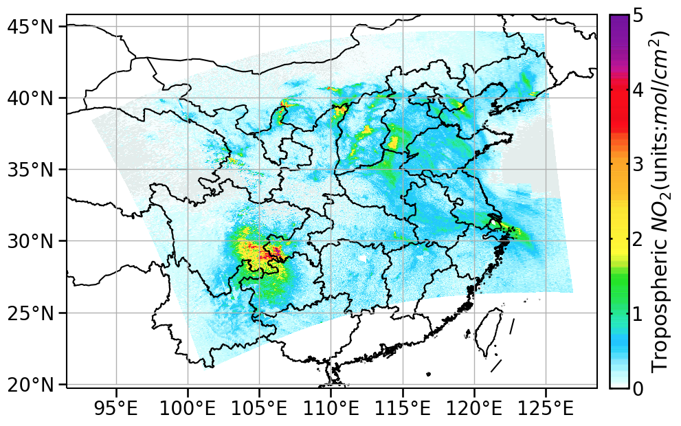
如果使用matplotlib中的pcolor/pcolormesh进行绘图的话，需要注意一点：pcolor和pcolormesh绘图时，所提供的x和y比C多1，即x和y应该是网格的边缘坐标，而不是中心坐标。具体见matplotlib官方的pcolormesh函数参数说明¹。

S5P的二级产品中提供了网格的边界坐标，但是需要简单的处理一下。处理代码如下(取自PyCAMA)：

 1
 2
 3
 4
 5
 6
 7
 8
 9
10
11
12
13
14
15
16
17
18
19
20
21
22
23
24
25
26
27
28
29
30
31
32
33
34
35
36
37
38
39
40
41
42
43
44
45
46
47


def prepare_geo(var, latb, lonb, selection="both"):
    if latb.shape[0] == 1:
        dest_shape = (latb.shape[1]+1, latb.shape[2]+1)
    else:
        dest_shape = (latb.shape[0]+1, latb.shape[1]+1)

    dest_lat = np.zeros(dest_shape, dtype=np.float64)
    dest_lon = np.zeros(dest_shape, dtype=np.float64)


    if latb.shape[0] == 1:
        dest_lat[0:-1, 0:-1] = latb[0, :, :, 0]
        dest_lon[0:-1, 0:-1] = lonb[0, :, :, 0]
        dest_lat[-1, 0:-1] = latb[0, -1, :, 3]
        dest_lon[-1, 0:-1] = lonb[0, -1, :, 3]
        dest_lat[0:-1, -1] = latb[0, :, -1, 1]
        dest_lon[0:-1, -1] = lonb[0, :, -1, 1]
        dest_lat[-1, -1] = latb[0, -1, -1, 2]
        dest_lon[-1, -1] = lonb[0, -1, -1, 2]
    else:
        dest_lat[0:-1, 0:-1] = latb[:, :, 0]
        dest_lon[0:-1, 0:-1] = lonb[:, :, 0]
        dest_lat[-1, 0:-1] = latb[-1, :, 3]
        dest_lon[-1, 0:-1] = lonb[-1, :, 3]
        dest_lat[0:-1, -1] = latb[:, -1, 1]
        dest_lon[0:-1, -1] = lonb[:, -1, 1]
        dest_lat[-1, -1] = latb[-1, -1, 2]
        dest_lon[-1, -1] = lonb[-1, -1, 2]

    boolarray = np.logical_or((dest_lon[0:-1, 0:-1]*dest_lon[1:, 0:-1]) < -100.0,
                              (dest_lon[0:-1, 0:-1]*dest_lon[0:-1, 1:]) < -100.0)

    if selection == "ascending":
        boolarray = np.logical_or(boolarray, dest_lat[0:-1, 0:-1] > dest_lat[1:, 0:-1])
    elif selection == "descending":
        boolarray = np.logical_or(boolarray, dest_lat[0:-1, 0:-1] < dest_lat[1:, 0:-1])
    else: # "both"
        pass

    dest_lon[0:-1, 0:-1] = np.where(boolarray, 2e20, dest_lon[0:-1, 0:-1])

    if var.shape[0] == 1:
        var = var[0, ...]
    else:
        var = var[...]

    return var, dest_lat, dest_lon

准备好以上代码之后就可以处理S5P二级产品了，示例代码如下：

 1
 2
 3
 4
 5
 6
 7
 8
 9
10
11
12
13
14
15
16
17
18
19
20
21
22
23
24
25
26
27
28
29
30
31
32
33
34
35
36
37
38
39
40
41
42
43
44
45
46
47
48
49
50


data = nc.Dataset('S5P_NRTI_L2__NO2____20200217T053859_20200217T054359_12156_01_010302_20200217T062043.nc')

prod = data.groups['PRODUCT']
lon = prod['longitude'][0,:]
lat = prod['latitude'][0,:]
no2 = prod['nitrogendioxide_tropospheric_column'][0,:,:]
qa_no2 = prod['qa_value'][0,:,:]
#no2[qa_no2 < 0.5 ] = np.nan

geopro = prod.groups['SUPPORT_DATA'].groups['GEOLOCATIONS']
geolon = geopro['longitude_bounds'][0]
geolat = geopro['latitude_bounds'][0]

no2, lat_bounds, lon_bounds = prepare_geo(no2, geolat, geolon)

fig, ax = plt.subplots(figsize=(12, 9), subplot_kw=dict(projection=ccrs.PlateCarree()))

ax.add_feature(cfeature.ShapelyFeature(china.geometries(), 
                                       ccrs.PlateCarree(), 
                                       facecolor='none', 
                                       edgecolor='k',
                                       linewidth=1.5))

con = ax.pcolormesh(lon_bounds,
                    lat_bounds,
                    no2*1e4, 
                    vmin=vmin, 
                    vmax=vmax, 
                    norm=aqi_norm, 
                    cmap=aqi_cmap)

lon_formatter = LongitudeFormatter(number_format=".0f",
                                   degree_symbol="",
                                   dateline_direction_label=True)
lat_formatter = LatitudeFormatter(number_format=".0f",
                                  degree_symbol="")

fig.canvas.draw()

ax.gridlines(xlocs=xticks, ylocs=yticks, linewidth=1, linestyles='--')
ax.xaxis.set_major_formatter(LONGITUDE_FORMATTER)
ax.yaxis.set_major_formatter(LATITUDE_FORMATTER)
lambert_xticks(ax, xticks)
lambert_yticks(ax, yticks)

cbar = fig.colorbar(con, ax=ax, shrink=0.9, pad=0.02)
cbar.set_ticks(ticks)
cbar.set_ticklabels(ticks)
cbar.ax.tick_params(direction='in', length=3, left=True, right=True)
cbar.ax.set_ylabel('Tropospheric $NO_2$(units:$mol/cm^2$)')

单轨道扫描NO2浓度分布

安装

下载源码后，使用如下方式解压并安装：

1
2
3


unzip PyCAMA.0.8.2.zip
cd PyCAMA-0.8.2
python setup.py install

测试是否安装成功，打开python/ipython

1

import pycama

或在终端执行如下命令：

1

python -c "import pycama; print(pycama.__version__)"

如果返回0.8.2则表示安装成功。

数据处理及可视化

生成配置文件

首先生成产品配置文件：

1

python PyCAMA_config_generator.py

脚本中有默认的配置文件名称，运行成功后会生成*.xml文件，生成之后为需要处理的产品生成数据处理配置文件：

1
2
3
4
5
6
7


python create_pycama_joborder.py -p NO2___ -m NRTI -c S5P*.xml -d /path/of/data/product/no2 -D 2020-02-17 -o no2_jobfile
# -p 表示需要处理的产品名称
# -m 表示数据的时间类型，即NRTI仅实时数据、OFFL离线数据等
# -c 表示前一步生辰的产品配置文件
# -d 表示产品的数据目录，以NO2为例
# -D 表示要处理的数据的日期
# -o 表示数据处理配置文件名称

上述两个脚本在PyCAMA-0.8.2/src目录下，可直接拷贝到指定的工作目录下使用。

生成三级产品

PyCAMA主要是通过配置文件的形式控制处理卫星多轨道扫描文件，将轨道扫描出现重叠的数据通过平均处理生成三级产品，同时提供了输出功能。以下是多轨道扫描文件的三级产品处理脚本：

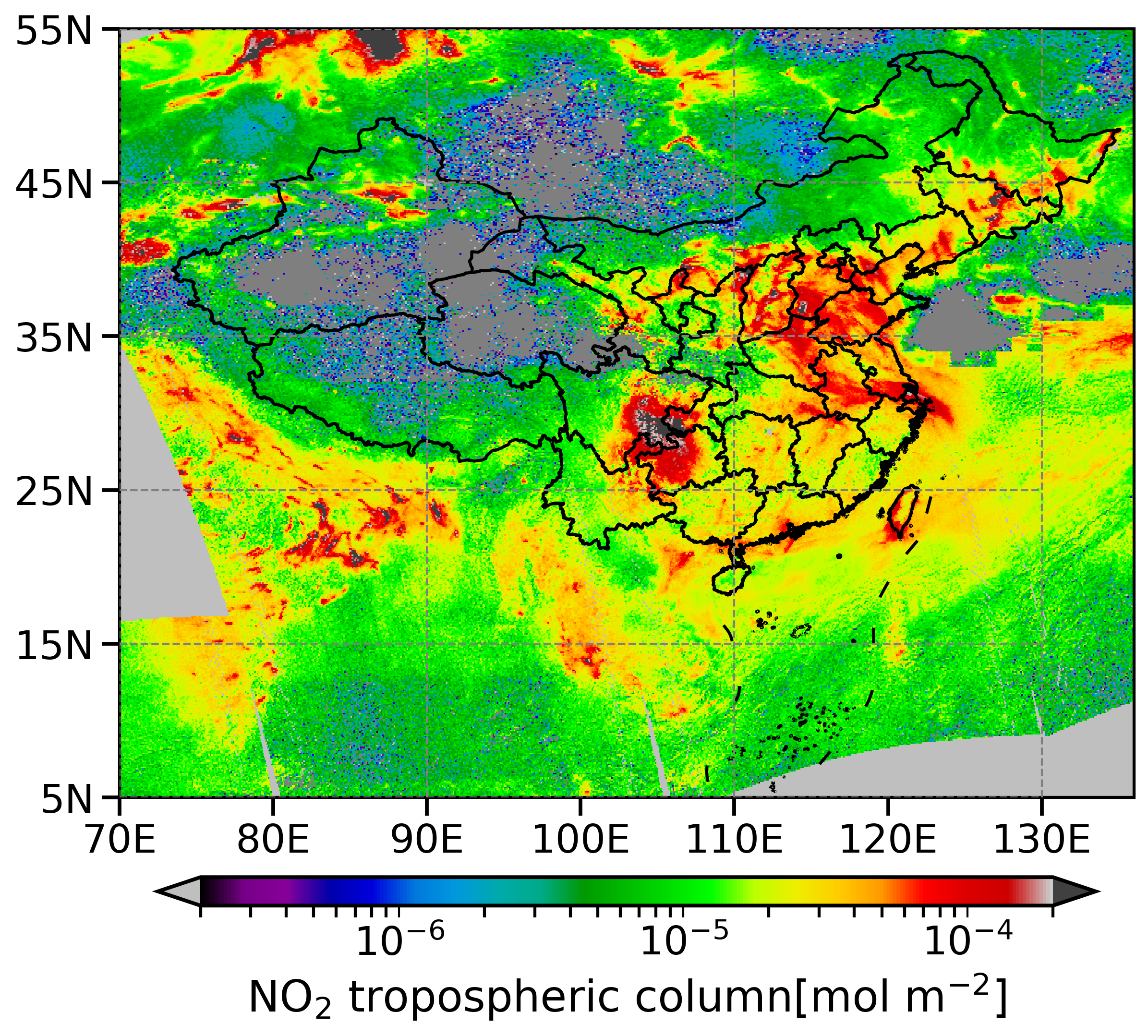
 1
 2
 3
 4
 5
 6
 7
 8
 9
10
11
12
13
14
15
16
17
18
19
20
21
22
23
24
25
26
27
28
29
30
31
32
33
34
35
36
37
38
39
40
41
42
43
44
45
46
47
48
49
50
51
52
53
54
55
56
57
58
59
60
61
62
63
64
65
66
67
68
69
70
71
72
73
74
75
76
77
78
79
80
81
82
83
84
85
86
87
88
89
90
91
92


import math
import numpy as np

import matplotlib as mpl
mpl.use('Agg')
from matplotlib import cm, ticker
from matplotlib.colors import LogNorm
import matplotlib.pyplot as plt

import cartopy.crs as ccrs
from cartopy.mpl.ticker import LongitudeFormatter, LatitudeFormatter
import cartopy.feature as cfeature
import cartopy.io.shapereader as shpreader

import seaborn as sns
from pycama import JobOrderParser, Reader, AnalysisAndPlot, Variable, WorldPlot

job = open('no2_jobfile')
joborder = JobOrderParser.JobOrder(job)
no2reader = Reader(joborder=joborder)

var = Variable(product='NO2___', field_name='nitrogendioxide_tropospheric_column', primary_var='nitrogendioxide_tropospheric_column')

no2reader.read()
data = WorldPlot(reader_data=no2reader, resolution=0.1)
data.process()

# 输出三级产品到指定文件
data.dump('no2_20200217.nc')

no2 =  {
        'color_scale': 'nipy_spectral',
        'data_range': [5.0e-06, 5.0e-4],
        'field_name': 'nitrogendioxide_total_column',
        'flag': False,
        'log_range': True,
        'primary_variable': 'nitrogendioxide_total_column',
        'show': True,
        'title': 'Total vertical NO\u2082 column',
        'units': 'mol/m\u00B2'
    }

## 提取需要绘图的变量
varname = 'nitrogendioxide_tropospheric_column'
plot_count = False

data_range = data.variables_meta[varname]['data_range']
normalizer = LogNorm(vmin=data_range[0], vmax=data_range[1])

if data.variables_meta[varname]['log_range']:
    fmt = ticker.LogFormatterMathtext(base=10.0, labelOnlyBase=False)
else:
    fmt = ticker.ScalarFormatter(useMathText=True)
    fmt.set_powerlimits((-3,3))
    
n_target = data.n_latitude*2*36
full_data_array = np.zeros((data.n_latitude, n_target), dtype=np.float64)

for i in range(data.latitude_centers.shape[0]):
    n = data.grid_length[i]
    ratio = n_target/n

    if plot_count:
        try:
            data_array = np.ma.asarray(self.data_for_latitude_band(i, varname, count=True))
            data_array.mask = (self.data_for_latitude_band(i, varname, count=True) == 0)
        except KeyError:
            print("Variable '{0}' could not be plotted".format(varname))
    else:
        try:
            data_array = np.ma.asarray(data.data_for_latitude_band(i, varname))
            data_array.mask = (data.data_for_latitude_band(i, varname, count=True) == 0)
        except KeyError:
            print("Variable '{0}' could not be plotted".format(varname))

    if np.all(data_array.mask):
        full_data_array[i, :] = np.nan
        continue

    for j in range(n):
        start_idx = int(math.floor(ratio*j+0.5))
        end_idx = int(math.floor(ratio*(j+1)+0.5))
        if data_array.mask[j]:
            full_data_array[i, start_idx:end_idx] = np.nan
        else:
            full_data_array[i, start_idx:end_idx] = data_array[j]
data._full_data_array = full_data_array

img = mapper.to_rgba(full_data_array)

data.graph_rep['data'] = img
data.graph_rep['name'] = varname

可视化

将多轨道卫星扫描数据生成三级产品后就可以画图了。以下是绘图脚本：

 1
 2
 3
 4
 5
 6
 7
 8
 9
10
11
12
13
14
15
16
17
18
19
20
21
22
23
24
25
26
27
28
29
30
31
32
33
34
35
36
37
38
39
40
41
42
43
44
45
46
47
48
49
50
51
52
53
54


### 开始绘图
china = shpreader.Reader('china.shp')

proj = ccrs.PlateCarree()
colormap = cm.get_cmap("nipy_spectral")
mapper = cm.ScalarMappable(norm=normalizer, cmap=colormap)

xstep, ystep = 10, 5
xmax, xmin, ymax, ymin = 135, 70, 5, 55
extent = [xmin, xmax, ymin, ymax]

fig, ax = plt.subplots(figsize=(12, 9), subplot_kw=dict(projection=proj))

con = ax.imshow(data.graph_rep['data'], origin='lower', extent=extent, transform=proj)

ax.set_extent([xmin, xmax, ymin, ymax], crs=proj)
yticks = np.arange(ymin, ymax+1, ystep)
xticks = np.arange(xmin, xmax+1, xstep)

ax.gridlines(xlocs=xticks, ylocs=yticks, crs=proj, linewidth=1, color='gray', linestyle='--', zorder=4)
ax.add_feature(cfeature.ShapelyFeature(china.geometries(),
                                       proj,
                                       facecolor='none',
                                       edgecolor='k',
                                       linewidth=1.))

lon_formatter = LongitudeFormatter(number_format=".0f",
                                   degree_symbol="",
                                   dateline_direction_label=True)
lat_formatter = LatitudeFormatter(number_format=".0f",
                                  degree_symbol="")

ax.set_xlim([xmin, xmax])
ax.set_ylim([ymin, ymax])
ax.set_xticks(np.arange(xmin, xmax+1, xstep))
ax.set_yticks(np.arange(ymin, ymax+1, ystep))
ax.set_xticklabels(np.arange(xmin, xmax+1, xstep))
ax.set_yticklabels(np.arange(ymin, ymax+1, ystep))
ax.xaxis.set_major_formatter(lon_formatter)
ax.yaxis.set_major_formatter(lat_formatter)

cbar = fig.colorbar(con, ax=ax, cmap=colormap,
                    norm=normalizer, extend='both', pad=0.08,
                    orientation='horizontal', shrink=0.9, aspect=30,
                    format=fmt)
ax1 = cbar.ax
ax1.clear()

cbar = mpl.colorbar.ColorbarBase(ax1, cmap=colormap, norm=normalizer, extend='both',
                                 orientation='horizontal', format=fmt)
cbar.ax.xaxis.set_tick_params(which='major', width=1.0, length=6.0, direction='out')
cbar.ax.set_xlabel('NO$_2$ tropospheric column[mol m$^{-2}$]')

fig.savefig('no2_20200217.png', dpi=100, bbox_inches='tight')

中国区域NO2浓度空间分布

注意事项

S5P卫星数据产品中提供了数据产品质量信息，在使用这些产品时应多加注意，根据应用需求对数据进行筛选。
使用netCDF4处理PyCAMA生成的三级产品输出文件时可能会报错，可以使用h5py进行处理。

https://matplotlib.org/3.1.3/api/_as_gen/matplotlib.pyplot.pcolormesh.html ↩︎